ZK-0: Arithmetic Circuits and mathematics involved in Zero-Knowledge Proofs
@shubh_exists|Aug 03, 2025 (10m ago)259 views
These are my notes while deep diving into zero knowledge proofs.
Understanding Problem Complexity Classes
Before diving into zero-knowledge proofs, we need to understand the different types of computational problems:
Problem Classifications
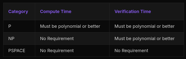
- P Problems - Problems that can be both solved and verified in polynomial time
- NP Problems - Problems that can be verified in polynomial time but might take exponential time to solve
- PSPACE Problems - Problems that require exponential resources to solve and verify
The Foundation of Zero-Knowledge Proofs
To verify any problem, we must express it as a boolean formula using logic gates (AND, OR, NOT). A solution that makes this formula true proves the problem statement is valid.
Key Insight: Zero-knowledge proofs only work with NP and P problems because these are efficiently verifiable. We assume the prover knows a solution to a boolean problem that only they can solve, while verification remains computationally feasible.
Without efficient verification, creating zero-knowledge proofs becomes infeasible.
Arithmetic Circuits: A More Efficient Approach
Binary circuits become unwieldy even for small problems, so we use arithmetic circuits to represent zero-knowledge proofs more efficiently.
What Are Arithmetic Circuits?
An arithmetic circuit is a system of equations using only three operations:
- Addition
- Multiplication
- Equality
Variables in arithmetic circuits are called signals.
Example:
6 = x₁ + x₂
9 = x₁x₂
This isn't an equation to solve—the user provides values to prove their knowledge, and we verify by substitution.
Why Arithmetic Circuits Matter
Many ZK algorithms (SNARK, STARK, Bulletproof) rely on arithmetic circuits because they:
- Translate naturally into Rank-1 Constraint Systems (R1CS)
- Provide a standard representation for zero-knowledge proofs
- Allow provers to assign arbitrary values to signals, with validity determined by constraint satisfaction
Practical Examples of Arithmetic Circuits
Example 1: 3-Coloring Australia

Problem: Color Australia's states with 3 colors so no adjacent states share the same color.
Solution Approach:
We assign numerical values to colors and create variables for each state:
- Blue → 1, Red → 2, Green → 3
- States: WA, SA, V, NT, Q, NSW
Step 1: Restrict each state to valid colors
0 === (1 - WA) * (2 - WA) * (3 - WA)
0 === (1 - SA) * (2 - SA) * (3 - SA)
0 === (1 - V) * (2 - V) * (3 - V)
0 === (1 - NT) * (2 - NT) * (3 - NT)
0 === (1 - Q) * (2 - Q) * (3 - Q)
0 === (1 - NSW) * (2 - NSW) * (3 - NSW)
Step 2: Ensure adjacent states have different colors
We use the property that multiplying two identical color values gives us products we want to avoid:
| State A | Adjacent State B | Product (A * B) | Is Selected? |
|---|---|---|---|
| 1 | 1 | 1 | No |
| 1 | 2 | 2 | Yes |
| 1 | 3 | 3 | Yes |
| 2 | 1 | 2 | Yes |
| 2 | 2 | 4 | No |
| 2 | 3 | 6 | Yes |
| 3 | 1 | 3 | Yes |
| 3 | 2 | 6 | Yes |
| 3 | 3 | 9 | No |
Products 1, 4, and 9 indicate same-color neighbors (invalid). Products 2, 3, and 6 indicate different-color neighbors (valid).
For neighboring pairs (WA,NT), (WA,SA), (SA,NT), (SA,Q), (SA,NSW), (SA,V), (NT,Q), (Q,NSW), (NSW,V):
0 === (2 - WA*NT)(3 - WA*NT)(6 - WA*NT)
0 === (2 - WA*SA)(3 - WA*SA)(6 - WA*SA)
0 === (2 - SA*NT)(3 - SA*NT)(6 - SA*NT)
0 === (2 - SA*Q)(3 - SA*Q)(6 - SA*Q)
0 === (2 - SA*NSW)(3 - SA*NSW)(6 - SA*NSW)
0 === (2 - SA*V)(3 - SA*V)(6 - SA*V)
0 === (2 - NT*Q)(3 - NT*Q)(6 - NT*Q)
0 === (2 - Q*NSW)(3 - Q*NSW)(6 - Q*NSW)
0 === (2 - NSW*V)(3 - NSW*V)(6 - NSW*V)
Example 2: Proving a List Is Sorted
Challenge: Prove every element is ≥ its predecessor using only addition, multiplication, and equality.
Key Insight: We convert numbers to binary and use the property that for n-bit elements, 2^n + (u-v) has MSB = 1 if and only if u ≥ v.
Solution for comparing two n-bit numbers u and v:
// Restrict u and v to n bits
u === 2^(n-1) * C(n-1) + 2^(n-2) * C(n-2) + ... + 2 * C(1) + C(0)
v === 2^(n-1) * D(n-1) + 2^(n-2) * D(n-2) + ... + 2 * D(1) + D(0)

// Ensure binary constraints
(C(n-1) - 1) * C(n-1) === 0
(C(n-2) - 1) * C(n-2) === 0
...
(C(0) - 1) * C(0) === 0

(D(n-1) - 1) * D(n-1) === 0
(D(n-2) - 1) * D(n-2) === 0
...
(D(0) - 1) * D(0) === 0

// Range check: 2^n + (u-v) should be (n+1)-bit number
2^n + (u - v) = 2^n * E(n) + 2^(n-1) * E(n-1) + ... + 2 * E(1) + E(0)

// Binary constraints for result
(E(n) - 1) * E(n) === 0
(E(n-1) - 1) * E(n-1) === 0
...
(E(0) - 1) * E(0) === 0

// MSB must be 1 for u ≥ v
E(n) === 1
This technique, called Range Checks, prevents numbers from exceeding specified bounds and is fundamental in ZKP systems.
Finite Fields: Solving Overflow and Precision Issues
Standard arithmetic circuits suffer from overflow and cannot represent fractions. Finite fields solve these problems.
What Is a Finite Field?
Given a prime number p, we create a finite field with p elements using integers {0, 1, 2, ..., p-1} where all operations are performed modulo p.
Key Properties:
- Order: The number of elements (p for prime fields)
- Equivalence: Numbers ≥ p or < 0 map to equivalent values in [0, p-1] via modulo p
- Common choice: p = 2²⁵⁵ - 19 (used in Curve25519)
Essential Finite Field Properties
Additive Operations
- Addition Identity: Adding p to any number yields the same result (equivalent to adding 0)
- Additive Inverse: For element a, the inverse is (p - a) mod p
Example in field with p = 7:
- Additive inverse of 3 is 4 (since 3 + 4 = 7 ≡ 0 mod 7)
- Additive inverse of 5 is 2 (since 5 + 2 = 7 ≡ 0 mod 7)
Multiplicative Operations
- Multiplicative Inverse: Every non-zero element a has inverse a⁻¹ where a × a⁻¹ = 1
- Exception: 0 has no multiplicative inverse
Example in field with p = 7:
- Multiplicative inverse of 3 is 5 (since 3 × 5 = 15 ≡ 1 mod 7)
- Multiplicative inverse of 2 is 4 (since 2 × 4 = 8 ≡ 1 mod 7)
Fermat's Little Theorem provides one method to compute inverses:
a^(p-1) ≡ 1 (mod p) for a ≠ 0
Therefore: a^(p-2) ≡ a^(-1) (mod p)
Advanced Properties
- Fractions: a/b = a × (multiplicative inverse of b)
- No Precision Loss: Division doesn't suffer from floating-point errors
- Algebraic Structure: Operations are associative, commutative, and distributive
- Square Roots: Not all elements have square roots (quadratic residues). I implemented tonelli-rs for computing modular square roots
Working with Systems of Equations
Finite field equation systems can have:
- No solution
- One solution
- p solutions (as many as the field order)
Importantly, real number solutions don't guarantee corresponding finite field solutions.
Polynomials in Finite Fields
Unlike continuous real polynomials, finite field polynomials are evaluated at discrete points only.
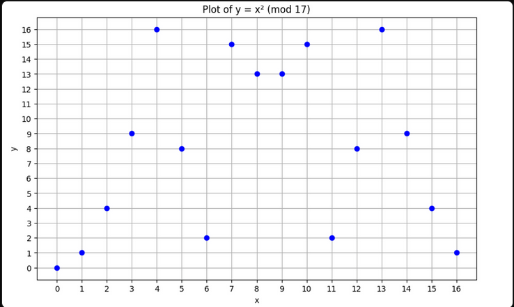
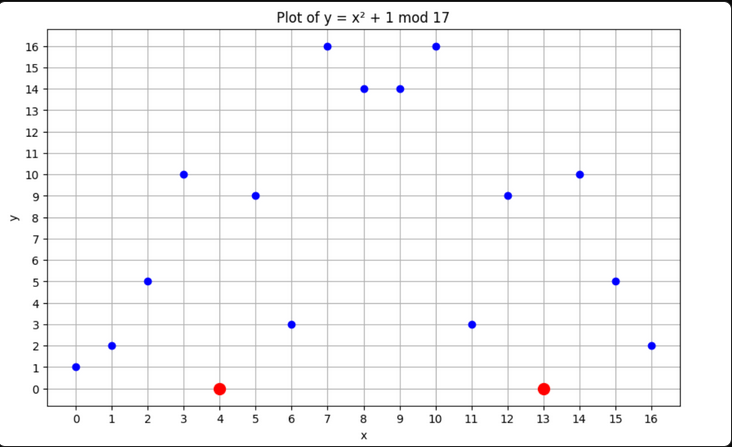
Surprising Result: Polynomials with no real roots may have finite field roots.
Example: y = x² + 1 has no real roots, but in a field of 17:
Popular cryptographic finite fields:
- BN254: Used in many Ethereum ZK applications
- BLS12-381: Used in newer protocols
- Goldilocks: p = 2⁶⁴ - 2³² + 1, optimized for 64-bit computers
Mathematical Foundations: Set Theory and Abstract Algebra
Elementary Set Theory
Functions establish mappings between input and output sets with the crucial restriction: each domain element maps to exactly one codomain element.
Valid mapping: (1,p), (2,q), (3,r)
Invalid mapping: (1,p) and (1,q) ← violates function uniqueness
Relations are any subset of the Cartesian product A × B.
Binary operators are functions A × A → B, taking two inputs from set A and producing one output.
Closed binary operators satisfy A × A → A (output remains in the same set).
Abstract Algebra Hierarchy
Abstract algebra studies sets with operators, classified by their behavioral properties:
Magma
- Definition: Set with a closed binary operator
- Requirement: Operation results stay within the set
Semigroup
- Definition: Magma with associative operator
- Requirement: a(b + c) = (a + b)c
Monoid
- Definition: Semigroup with identity element
- Requirement: ∃e such that a × e = e × a = a
Group
- Definition: Monoid where every element has an inverse
- Requirements:
- Closed operation (Magma)
- Associative operation (Semigroup)
- Identity element (Monoid)
- Every element has an inverse
Abelian Groups
- Additional Property: Commutative operation (a × b = b × a)
Elementary Group Theory
Finite Groups
Groups with finite element counts. The order of a group is its element count.
Example: Integer addition modulo a prime forms a finite group.
Cyclic Groups
Groups where every element can be generated by repeatedly applying the operator to a single generator element.
Key Property: All cyclic groups are abelian.
Examples:
Addition modulo 7 (cyclic):

Multiplication modulo 7 (excluding zero):
-
Generator 2:
Generator 2 does not generate all elements.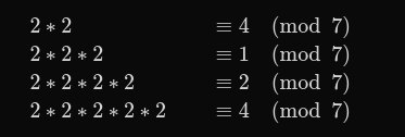
-
Generator 3:
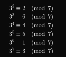
Generator 3 generates all elements because 3 is a primitive root.
Important: Group identity elements are unique.
Homomorphisms: Structure-Preserving Maps
Definition
A homomorphism between groups G and H is a function φ: G → H that preserves the group operation:
φ(a ⋅ b) = φ(a) ∗ φ(b)
Example
Consider:
- G = (ℤ, +): integers under addition
- H = (ℤₙ, +): integers modulo n under addition
Define φ: ℤ → ℤₙ by φ(k) = k mod n
Then: φ(a + b) = (a + b) mod n = (a mod n + b mod n) mod n = φ(a) + φ(b)
Key Properties
- Identity preservation: φ(eG) = eH
- Inverse preservation: φ(g⁻¹) = φ(g)⁻¹
- Image is subgroup: φ(G) ⊆ H forms a subgroup
- Kernel:
ker(φ) = {g ∈ G | φ(g) = eH}measures information loss
Cryptographic Significance
Crucial insight: "Elliptic curve points in a finite field under addition form a finite cyclic group that is homomorphic to integers under addition."
Homomorphisms enable homomorphic encryption: if φ: A → B is hard to invert, we can validate claims about computations in A using elements in B.
Elliptic Curves: The Foundation of Modern Cryptography
Basic Definition
Elliptic curves follow the equation:
y² = x³ + ax + b
In finite fields:
y² ≡ (x³ + ax + b) (mod p)
Requirements
- a, b ∈ F (the field)
- 4a³ + 27b² ≠ 0 (ensures non-singularity—tangents exist at all points)
Geometric Properties
- Symmetry: Always symmetric about the x-axis
- Intersections: Meets x-axis at 1-3 points maximum
Group Operations
Point Addition
For points P(x₁, y₁) and Q(x₂, y₂):
- Draw line PQ
- Find third intersection point R with the curve
- Reflect R across x-axis to get P + Q
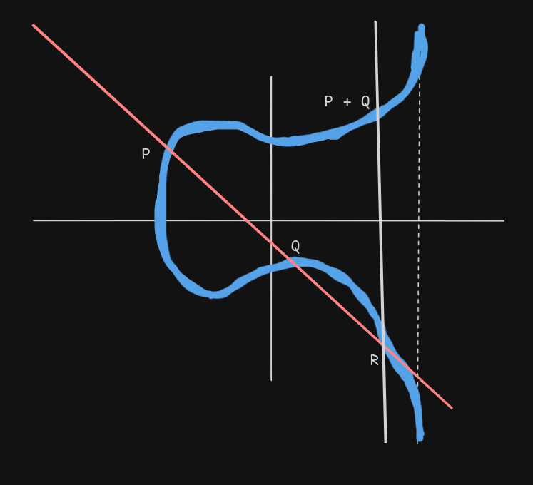
Formulas:
s = (y₂ - y₁)/(x₂ - x₁) (mod p)
x₃ ≡ (s² - x₁ - x₂) (mod p)
y₃ ≡ (s(x₁ - x₃) - y₁) (mod p)
Point Doubling
For point P(x₁, y₁) to compute 2P:
- Draw tangent at P
- Find second intersection Q with curve
- Reflect Q across x-axis to get 2P
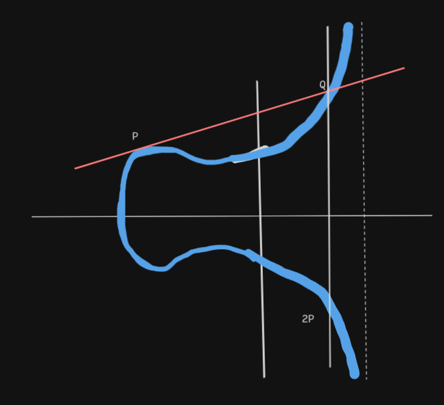
Formulas:
s = (3x₁² + a)/(2y₁) (mod p)
x₃ ≡ (s² - 2x₁) (mod p)
y₃ ≡ (s(x₁ - x₃) - y₁) (mod p)
Efficient Scalar Multiplication: Double-and-Add
To compute kP efficiently:
- Convert k to binary: k = (bₘ₋₁bₘ₋₂...b₁b₀)₂
- Initialize R = P (start with MSB)
- For each remaining bit (MSB-1 down to LSB):
- Double: R = 2R
- If bit = 1: Add: R = R + P
- Result: R = kP
The Discrete Logarithm Problem
Given:
- Elliptic curve: y² = x³ + ax + b (mod p)
- Group order: |E(Fₚ)| = n
- Generator point P
- Point R
Problem: Find integer x where 1 ≤ x ≤ n such that:
xP = R
Asymmetry:
- Easy: Computing R given x (forward direction)
- Hard: Computing x given R (inverse/discrete logarithm)
This asymmetry enables elliptic curve cryptography.
Zero-Knowledge with Elliptic Curves
Claim: "I know values x and y such that x + y = 15"
Protocol:
- Prover: Computes A = xG and B = yG (where G is generator)
- Prover: Sends A and B to verifier
- Verifier: Computes 15G and checks that A + B = 15G
Security: Without knowing x or y, the verifier can confirm the sum relationship while learning nothing about the individual values.
This comprehensive guide covers the mathematical foundations essential for understanding zero-knowledge proofs, from basic arithmetic circuits through the elliptic curve cryptography that powers modern ZK systems.